Executive Summary

• The Parcl Price Feed V2 (PLPF V2) is the first price feed of its kind that allows users to track daily price movements across more than different geographies and housing segments such as all housing units, single family homes and new construction units. The PLPF V2 allows our users to understand and compare market conditions using a simple, accessible measure: price per square foot.

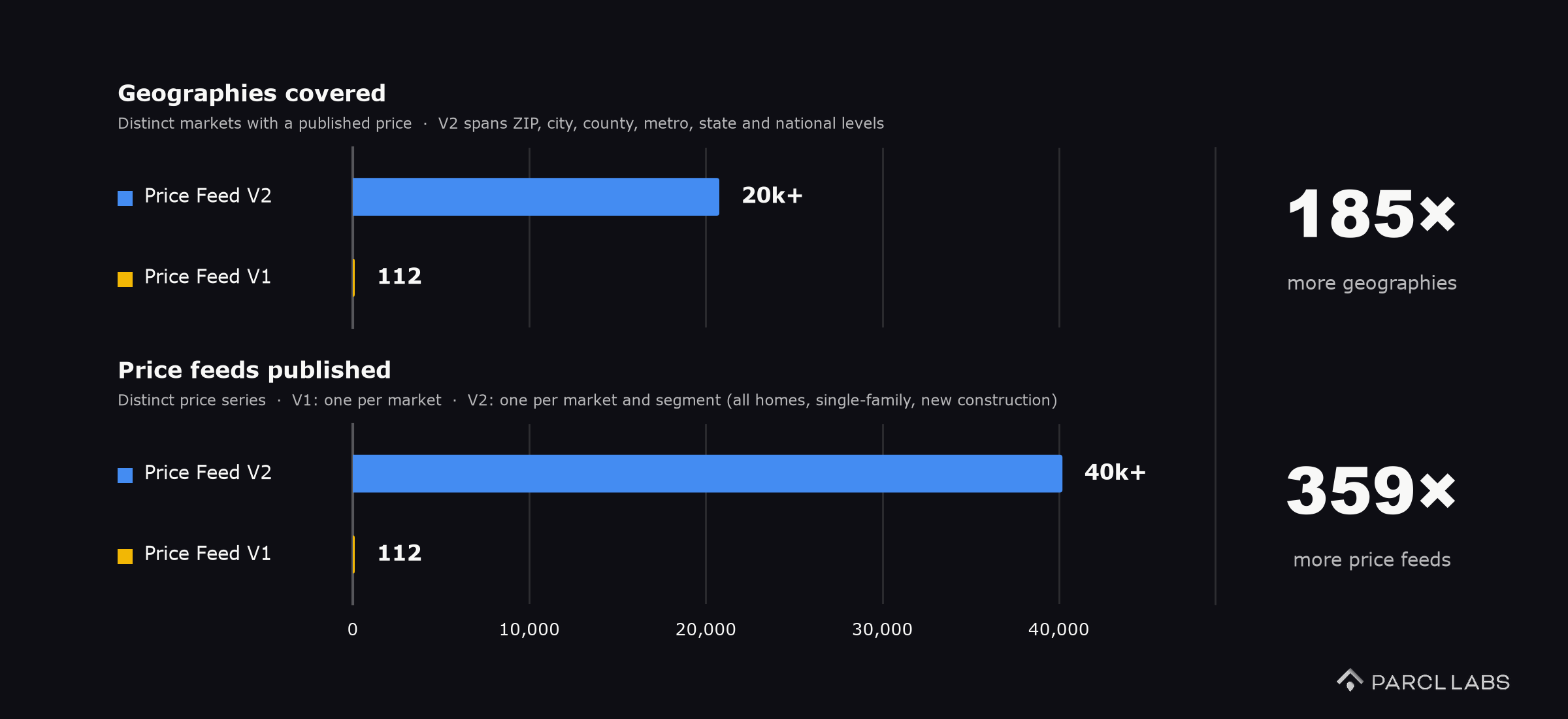
• The PLPF V2 covers more than 20k geographies, from ZIP codes to the country, and publishes more than 40k unique price feeds across them. This scale is made possible by a revamped methodology optimized for thin markets, where data is sparse or slow to arrive.

• Our PLPF V2 introduces several methodological improvements that allow us to provide more robust and resilient price feeds: chained price estimates with corrections toward observed price levels; thin markets use movement from a broader hierarchical geographic area; indices use more robust outlier detection filters; and improved sample spaces using dynamic windows tailored to markets and segments to increase coverage.

• We also increased the coverage and quantity of the data used in our estimates with over 400 million different data points available in the creation of our indices. Our new price feed provides a never-before-seen level of detail by breaking price movements across segments, allowing for a more accurate reading of the real estate markets.

• The PLPF V2 empowers users to make better informed decisions and can be accessed through our user-friendly API.

Introduction

Residential real estate data lives in silos, is lagged, sometimes only reflects a small sliver of the market, and has a high degree of heterogeneity from source to source. When we launched the first version of our PLPF we tried to solve those challenges to provide timely real estate insights across a wide variety of markets. The first version of our feed allowed our customers to get timely and reliable information, but it also showed us that a more refined version was possible.

One of the critical realizations was that, although we could provide the most up-to-date and accurate price estimate for a wide variety of markets, for geographies with a lack of sufficient timely data a robust estimator was not accurate enough with our original methodology. The problem of thin markets was compounded by the lack of timeliness of some official government data, where some transactions would become available more than 2 years after the sale closed.

We also observed how price dynamics can differ greatly within a single market once we look at segments. In Boston, the overall market and single family homes are moving in opposite directions. As of September 10, the PLPF V2 shows all homes down about 6.5% year over year while single family homes are up more than 8%. Syracuse shows the same split with the pattern reversed. The PLPF V2 has all homes up 16.4% year over year against 8.3% for single family homes, a gap explained by the much faster appreciation of townhouse stock relative to single family homes. A single market number would miss both stories.

Figure 1. Price Feed V2 by Segments in Boston

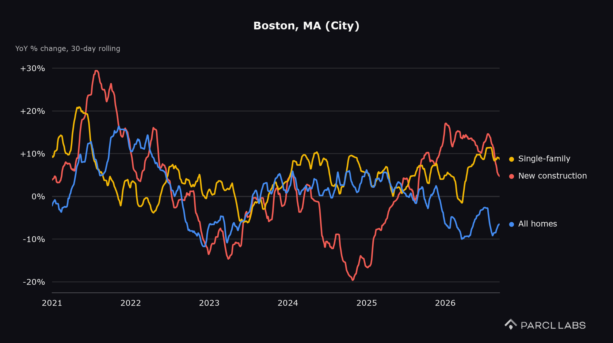
The PLPF V2 builds on the work behind our original feed to address these challenges. It keeps what our users valued in the first version, the simple metric, the daily cadence and a look-back window that adapts to each market, and it extends the feed so that our users can:

• Have reliable feeds for a wider variety of geographies, including thin markets. We have custom windows with dynamic limits that allow a series to look back in time when a market has low volume, so there are enough observations to estimate from. Better filters remove outliers relative to each window and give more weight to the most recent prices, so a longer window does not mean a stale or noisy estimate. And when activity dries up altogether, a market draws on the movement of the larger geography that contains it, so a ZIP code can lean on its county/city through a thin period and return to its own data when sales pick up.

• Understand segments in a market. Different types of homes respond to different forces. Condos and townhomes trade on a different buyer pool and a different supply than single family homes, and new construction follows builder pricing and incentives more than the resale market. When all of them are pooled into one number, those dynamics hide behind the mix of what happened to sell that month. V2 estimates and publishes all housing units, single family homes and new construction as separate series for every market, so our users can see which part of a market is moving and read housing dynamics across unit types instead of an average of them.

• Observe market movements before all the records catch up. Evidence about a market arrives at different speeds: listings show where sellers are pricing today, reported sales follow within weeks, and the official record of a closing can take months or years. The PLPF V2 separates two questions. How much did the market move today is answered by the freshest evidence available, and where does the market sit is answered by closed sales. The index chains the daily movements and is continuously corrected toward the level that closed sales support, so a late batch of records refines the level gradually instead of resetting it.

Together these changes uncover a view of residential real estate that did not exist before: a daily price per square foot for more than 20k geographies, from the ZIP code to the country, each broken into segments, and all measured the same way. A user can watch a single ZIP code reprice week by week, compare it with its county and its metropolitan area on the same scale, and see what segment is driving the move.

Figure 2. Coverage Increase between Price Feed V1 and V2

Data

The first version of the PLPF was built on sales and listings from a handful of sources. For V2 we widened that base to include almost half a billion data points, including sales from county registrars, tax assessors, website aggregators, listings, and other online sources. More data is only useful if it describes the same homes consistently, so every record goes through the enrichment process we use across Parcl before it can reach the estimator:

• One record per property. Addresses arrive in many spellings, and the same home can appear in several sources under several of them. We clean, standardize and de-duplicate addresses to build a single source of truth for each property, and we validate that record against a third party to guarantee its integrity.

• Reconciled attributes, refreshed daily. Sources disagree about a home: one may hold it at 1,700 square feet and another at 1,600. A reconciliation process compares the sources and time periods available for each property and settles on the most reliable value. It runs daily across all of our properties, so the estimator always works from the latest view of each home, and every price per square foot in the PLPF is computed on that reconciled size.

• Placed in every market it belongs to. Using spatial data science we assign each property to its ZIP code, city, county, metropolitan area and state, so one sale informs up to six markets and the feed can be built at whichever level of geography a user needs.

The observation universe includes all property types (single family homes, townhomes, condos, semi-detached, etc.) and also differentiates between new construction and existing stock. This provides a level of granularity that allows us to create very detailed price feeds across segments and geographies.

Parcl Labs Price Feed V2 Methodology

The PLPF V1 used a look-back window tailored to a market's transaction volume, so that a busy market was read from its recent sales and a quieter one reached further back, using a reduced sample space of observations between the 35th and 65th percentiles. To reduce day-to-day noise we added a smoothing factor to effectively create a rolling average of the median prices we observed. The second version of our PLPF follows a similar approach with several new features.

Dynamic Tailored Look-back Windows

In the PLPF V1 different markets already had different windows, sized by their transaction volume, to account for smaller markets. V2 turns that into a formula that every market, segment and type of evidence applies every day. Let $\mathcal{I}_k(t, W) = \{ i : t - W < \tau_i \le t \}$ be the observations of type $k$ (listings, sales, etc.) in the $W$ days ending on day $t$. The window is the shortest one, in increments of five days, that holds enough observations such that:

$$W_{k,t} = \min\left\{ W \in \{30, 35, \ldots, 180\} : \left|\mathcal{I}_k(t, W)\right| \ge N_{g,k} \right\}$$

where the target $N_{g,k}$ grows with the size of the geography and is three times larger for listings than for sales. In this way we establish a different minimum requirement for metros, counties, cities and ZIP codes (represented by $g$). This allows a market with lots of transactions to only reach back for a handful of days while a small ZIP code may need to reach back for a longer window. We established a hard limit of 180 days to prevent stale prices from propagating forward. Since we are looking at smaller geographies where small data entry errors can have a disproportionate impact on price estimates we add another filter. Once the window $W_{k,t}$ has been selected, we take the median price per square foot of everything inside it and call it $m_0$. That median is the window's own reading of a typical home. We then keep only the observations whose price per square foot $p_i$ lies between 45% and 220% of it:

$$\mathcal{B}_{k,t} = \left\{ i \in \mathcal{I}_k(t, W_{k,t}) : 0.45\, m_0 \le p_i \le 2.2\, m_0 \right\}$$

Here $\mathcal{I}_k(t, W_{k,t})$ is the set of observations of type $k$ inside the chosen window, and $\mathcal{B}_{k,t}$ is the subset that survives the filter and goes on to the next step. Because the band is measured against the window's own median, it adapts to each market and moves with it, working by transaction type, so that neither sales nor other types of observations, like listings, have a disproportionate impact on the estimate.

Recency Weighted Median with Decaying Factor

A trade-off that arises when we increase the window size is that a sample space can suddenly carry data from a distant period of time. To prevent older records from having an undue influence on our price estimates we use decaying weights where an observation loses half its weight each time its age grows by half the window, and the estimate describes the market as it stands today even when the window is long. This is described by:

$$w_i = 2^{-a_i / h_{k,t}}, \qquad h_{k,t} = \max\left(W_{k,t} / 2,\; 7\right)$$

where $w_i$ is the weight assigned to observation $i$, $a_i = t - \tau_i$ is the number of days since that observation occurred (event date), and $h_{k,t}$ is the half-life, the number of days it takes for a weight to fall by half. The half-life is set to half the window $W_{k,t}$ chosen in the previous step, with a floor of seven days so that even the shortest window does not discount a sale that is a few days old. This allows the PLPF V2 to give more weight to recent transactions and retain observations that support robust price readings, while ensuring that older transactions have less influence on the price estimates.

One more adjustment protects the estimate from a single day. Builders and recording offices often post many closings at once, and in a small window such a batch can look like a price move. Let $n_d$ be the number of retained observations dated $d$ and $\bar{n}_{k,t}$ the average number of observations per day over the trailing year. With the cap $c_{k,t} = \max(4,\; 1.5\, \bar{n}_{k,t})$,

$$\tilde{w}_i = w_i \, \min\left(1,\; \frac{c_{k,t}}{n_{d(i)}}\right)$$

so a day with more observations than the cap counts as if it held exactly $c_{k,t}$ of them. $\tilde{w}_i$ is the final weight an observation carries into the median.

After selecting the window and applying the outlier filter, each surviving observation carries a price per square foot and a weight. Recency weighting gives newer observations more influence. In the PLPF V1, the sales estimate was an unweighted median of observations between the 35th and 65th percentiles. V2 uses weighted percentiles and a weighted median. We sort observations from lowest to highest price per square foot and calculate their total weight. Starting at the lowest price, we add each observation’s weight to a running total. We keep an observation when that running total falls between 20% and 75% of the total weight, that is, between the 20th and 75th weighted percentiles, using the 35th to 65th percentiles for listings in non-disclosure markets. We then calculate the combined weight of the retained observations and reset the running total to zero. Moving through the retained observations in price order, we add their weights again. The first price where the running total reaches or exceeds half of the retained weight is the weighted median. This becomes the initial daily estimate for that source within the market and housing segment. If percentile trimming would leave fewer than three observations, we skip that trimming step and calculate the weighted median using all observations that passed the earlier outlier filter, keeping their recency and daily-cap weights.

Formally, with the observations sorted by price, $p_{(1)} \le \cdots \le p_{(n)}$, and $C_j = \sum_{l \le j} \tilde{w}_{(l)}$ the running total of weight up to position $j$, the retained set and the daily estimate are:

$$\mathcal{T}_{k,t} = \left\{ j : 0.20\, C_n \le C_j \le 0.75\, C_n \right\}$$

$$\tilde{L}_{k,t} = p_{(j^{*})}, \qquad j^{*} = \min\left\{ j \in \mathcal{T}_{k,t} : \sum_{l \in \mathcal{T}_{k,t},\, l \le j} \tilde{w}_{(l)} \;\ge\; \tfrac{1}{2} \sum_{l \in \mathcal{T}_{k,t}} \tilde{w}_{(l)} \right\}$$

where $C_n$ is the total weight in the window, $\mathcal{T}_{k,t}$ is the set of retained positions, and $j^{*}$ is the first retained position at which the running total of retained weight reaches half of the retained total. A level is produced only when the window holds at least five observations.

Three properties make this a better estimate than an average, or than a plain median. First, it does not care how extreme the extremes are. Second, it reads the market where the data is densest. The estimate lands near the 47.5th percentile of the weighted distribution, close to the midpoint of the band, and the precision of any percentile estimate depends on how many homes are priced close to it. Finally, because the median is taken by weight, it inherits the recency decay and the daily cap from the previous step, so the result describes the market today and not the average of the last several months.

Chained Returns

After these steps we have distributions for sales and listings, but those series do not agree on what the price per square foot should be. Sales tell us where prices really are, but they arrive late, in some counties years after the transaction. Listings tell us where sellers are pricing this week, but they are asking prices and not closings. In the PLPF V1 we resolved this by blending a sales median and a listing median with different weights. That works in markets with enough sales volume, but it is not as robust in markets with low sales volume.

The PLPF V2 solves this challenge with chained returns applied to a starting price level. We begin by calculating the initial price level for a given market using sales as the main indicator to set the level. From then on, each day we take the daily levels from the previous step and compute each source's change from its own previous level. These changes are combined using source weights that reflect reliability and typical observation counts. The model averages the contributing sources logarithmic changes, accounting for gaps in the time series and limiting unusually large movements, and applies the combined movement to the previous chain level. For example, a level of 200 dollars per square foot followed by increases of 1% and 2% becomes 202 dollars and then 206.04 dollars. Each day therefore builds on the preceding level, creating the chain. After this update, the model can make a gradual correction toward the price levels supported by current observations. The chain level and the previous source estimates are carried forward so that the next day continues from that point.

The change of source $k$ on day $t$ is its daily log return, and the chain level $P_t$ advances by the weighted average of those returns before the separate correction toward observed price levels:

$$r_{k,t} = \frac{\ln L_{k,t} - \ln L_{k,s}}{t - s}$$

Here, $r_{k,t}$ is the average daily log return for source $k$ within a particular market and housing segment. $L_{k,t}$ is the source's price per square foot on day $t$, and $L_{k,s}$ is its previous available estimate, produced on day $s$. The difference between their natural logarithms, $\ln(L_{k,t}) − \ln(L_{k,s})$, measures the proportional change between the two estimates. Dividing by $t − s$, the number of calendar days between them, converts that change into a daily rate allowing us to put changes measured over different time intervals on the same daily scale.

Once we have this we then combine the returns across sources with the formula:

$$\qquad r_t = \frac{\sum_{k \in \mathcal{A}_t} \omega_k \, r_{k,t}}{\sum_{k \in \mathcal{A}_t} \omega_k}$$

where $r_t$ stands for the combined daily log return across the sources contributing on day $t$, $A_t$ is the set of contributing sources, and $\omega_k$ is the weight assigned to source $k$. We multiply each source's daily log return $r_{k,t}$ by its weight, add those weighted returns, and divide by the total weight of the contributing sources. The weight $\omega_k$ determines how much the price movement of source $k$ influences the combined movement. It is calculated as:

$$\omega_k=\theta_k\bar N_k$$

where $\bar N_k$ is the source’s average number of observations per window and $\theta_k$ is its reliability factor. A source with more observations or a higher reliability factor receives more influence. For example, if sales have a weight of 30 and listings have a weight of 10, sales receive 75% of the influence and listings receive 25%. The model uses these shares to average their logarithmic price changes. The baseline weights remain fixed during ordinary daily updates, but the shares can change when a source cannot contribute. If only sales contribute, they receive 100% of the influence. These weights control how price changes are combined; they do not discount the underlying prices.

After we get the daily rate we add an extra layer of scrutiny to guarantee that unusual price swings do not alter the price estimates. We cap this return component at ±0.02 log units per day covered:

$$\ln P_t=\ln P_{t-1} +clip(r_t c_t, -0.02c_t, +0.02c_t)$$

Where $c_t$ is the number of days covered by the update: the smallest of the days since the chain’s last return update, the largest gap among contributing source estimates, and 45 days. The clip function keeps the applied movement within these limits.

A chain of returns keeps the index moving with the market, but on its own it says nothing about whether the level is right. Listings can run ahead of closings for months, a market's recorded sales can land in a batch long after the fact, and each of those leaves a gap between the chain and the prices on the deeds. The PLPF V2 adjusts the series to minimize any level deviation on a continuous basis. After every daily movement, the chain is compared with the level that the sales in the window support and moved a small step toward it using this formula:

$$\ln P_t \leftarrow \ln P_t + \gamma_t \left( \ln T_t - \ln P_t \right)$$

where $T_t$ is the target level, the average of the sales levels in the window weighted by how many sales each one holds, and $\gamma_t$ is the fraction of the gap closed on day $t$. The fraction $\gamma_t$ is small, about 1% of the gap per day or less, and three rules govern it. First, it follows the evidence. With twenty or more sales in the window the correction runs at full strength, with fewer it is weaker, and with fewer than five sales it is not applied. In that last case the listing level, adjusted by the market's sale-to-list ratio, stands in as the target with a reduced pull. Second, it does not switch off. If the chain drifts from the level that sales support, a minimum pull remains so the gap keeps closing. Third, it is capped. Once a series has a long history the correction is limited to 10% a year, so a single unusual batch of closings cannot swing an established market.

On any single day the correction is too small to modify the price movements in the PLPF V2, but over an extended period of time it helps keep the feed tied to real price levels.

Parent Market Smoothing

Even with a window of up to 180 days and using both listings and sales, small markets can have extended periods with little new evidence to inform price movements. The new price feed uses the hierarchical and spatially correlated nature of real estate prices and uses larger geographies to fill in price movements when markets are too thin.

What a small market does have is a neighbor that is measured well. Prices in a ZIP code move largely with its county, and a county with its metropolitan area. The PLPF V2 uses that relationship to fill the holes. Each market below the state has a parent: a ZIP code or city reports to its county, a county to its metropolitan area, and a metropolitan area to its state, with the next broader geography stepping in when the usual parent has no estimate. States and the country stand on their own evidence.

For markets with an available parent return, the filter first follows the parent’s movement and then adjusts toward the market’s own estimate. The strength of that adjustment depends on the amount of local evidence. Here, $\Pi_t$ is the parent’s smoothed model index, $P_t$ is the market’s own chained index before this smoothing step, and ℓₜ is the market’s smoothed level expressed as a natural logarithm. First, we calculate the parent’s log change and limit the movement passed to the market to ±0.02 logarithmic units:

$$d_t = \operatorname{clip}\left( \ln \Pi_t - \ln \Pi_{t-1},\; \pm 0.02 \right)$$

then we add that movement to the market’s previous smoothed log level to obtain a preliminary estimate. The equation $\hat{\ell}_t = \ell_{t-1} + d_t$ defines the market’s preliminary estimate for day $t$ and $\ell_{t-1}$ is the market’s previous smoothed log level, and $d_t$ is the parent’s log change after clipping. Adding them moves the market’s previous level by the parent’s proportional movement. The hat in $\hat{\ell}_t$ indicates that this is an intermediate estimate, before adjusting toward the market’s own data described by the equation:

$$\ell_t = \hat{\ell}_t + \kappa_g \, \frac{n_t}{n_t + K_g} \, \operatorname{clip}\left( \ln P_t - \hat{\ell}_t,\; \pm 0.10 \right)$$

This equation takes the preliminary estimate $\hat{\ell}_t$ and adjusts it toward the market’s own chained index $P_t$. The difference $\ln P_t-\hat{\ell}_t$ measures the gap between the market's own chained index and the parent-driven preliminary estimate in log terms. We first limit that gap to between −0.10 and +0.10, then multiply it by $\kappa_g \frac{n_t}{n_t + K_g}$ to determine how much of the gap to close. Here, $n_t$ is the market’s effective observation count, $K_g$ controls how strongly limited data reduces the adjustment, and $\kappa_g$ sets its maximum rate for geography type $g$. Adding this adjustment to $\hat{\ell}_t$ gives the updated smoothed log level $\ell_t$. If the market’s own estimate is higher, the adjustment raises the preliminary level; if it is lower, the adjustment reduces it.

Here $n_t$ is the market's effective number of observations, its sales plus its listings counted at 0.30 each, or 0.60 in non-disclosure markets. The constants depend on the level of geography.

Table 1. Parent Market Smoothing Parameters by Geography

There is a simple way to read this filter. Write $u_t = \ell_t - \ln \Pi_t$ for the market's premium over its parent in logs, and $\eta_t = \kappa_g \, n_t / (n_t + K_g)$ for the gain. When neither limit binds, the update above is the same as:

$$u_t = u_{t-1} + \eta_t \left( \left( \ln P_t - \ln \Pi_t \right) - u_{t-1} \right)$$

Put simply, a market moves with its parent, plus the change in its own premium, and that premium is learned from the market's own data at a speed set by how much data is available. The market keeps its own price level. A ZIP code that is 30% more expensive than its county stays 30% more expensive. What it borrows is the day-to-day movement. With a constant observation count and target premium, daily updates, and when neither clipping limit binds, a ZIP code with ten effective observations has a gain of 0.007 and takes about 97 days to close half of a gap between what its own data says and what the feed shows. With sixty observations that takes about 27 days, and with three hundred about 16. So a thin market follows its county closely, a deep market follows its own evidence, and the transition between the two is gradual, with no cliff where a market suddenly switches method. When its own raw index is unavailable, an initialized market can continue with the parent’s movement, if available. Publication still depends on local evidence and quality requirements.

Non-Disclosure States

In some states sale prices are not part of the public record. The amounts attached to recorded sales in those states are not closing prices but estimates, typically derived from the mortgage, and the way they are derived can change without notice. Left alone, such a change reads in the feed as a price movement that never happened, and because it applies to a whole state at once it reaches every market inside it. V2 therefore rescales these amounts before they enter the estimator, using two things we can observe for the same home: what it was listed for, and the mortgage recorded with it.

For each recorded sale we find the most recent listing of the same property in the preceding months and form the ratio of the recorded amount to the asking price. Let $R_{s,m}$ be the median of those ratios in state $s$ and month $m$, and $\bar{R}_{s,m}$ a short exponentially weighted average of the most recent months, where a month with too few matched pairs carries the last measured value forward. As a benchmark we use the mortgage. With an assumed loan-to-value ratio $v$, a first mortgage of amount $m_i$ implies a price of $m_i / v$, and $R^{*}_s$ is the average ratio of that implied price to the asking price over the last several years in state $s$. The adjustment factor is

$$\phi_{s,m} = \operatorname{clip}\left(\frac{R^{*}_s}{\bar{R}_{s,m}},\; \phi_{\min},\; \phi_{\max}\right)$$

and the amount of a recorded sale in state $s$ and month $m$ is multiplied by $\phi_{s,m}$ before its price per square foot is computed. When recorded amounts drift down relative to asking prices, $\bar{R}$ falls and $\phi$ rises, which brings the amounts back to the mortgage-anchored baseline. The factor is bounded, and it is set to one when either ratio is unavailable.

We tested the adjustment where the answer is known. In disclosure states the true sale price is public, so we assembled 18.9 million recorded sales with a matched mortgage across 38 disclosure states, from January 2019 through August 2026, 7.5 million of which also matched a listing of the same home in the preceding 180 days. We replaced their recorded prices with mortgage-derived amounts of the kind we receive in non-disclosure states, ran the adjustment over a grid of 44 parameter settings with states and time periods held out from tuning, and compared the results with the prices actually recorded. On every holdout the adjusted amounts were closer to the recorded prices than the unadjusted ones, both for individual sales and for the level of the market. Beyond the adjustment, markets that are predominantly non-disclosure run under more stringent limits: listings are trimmed to the narrower 35th to 65th percentile band, listing movements carry more weight and recorded sales less, and reported sales that can echo the asking price are excluded.

Table 2. Parcl Price Feed V1 vs V2

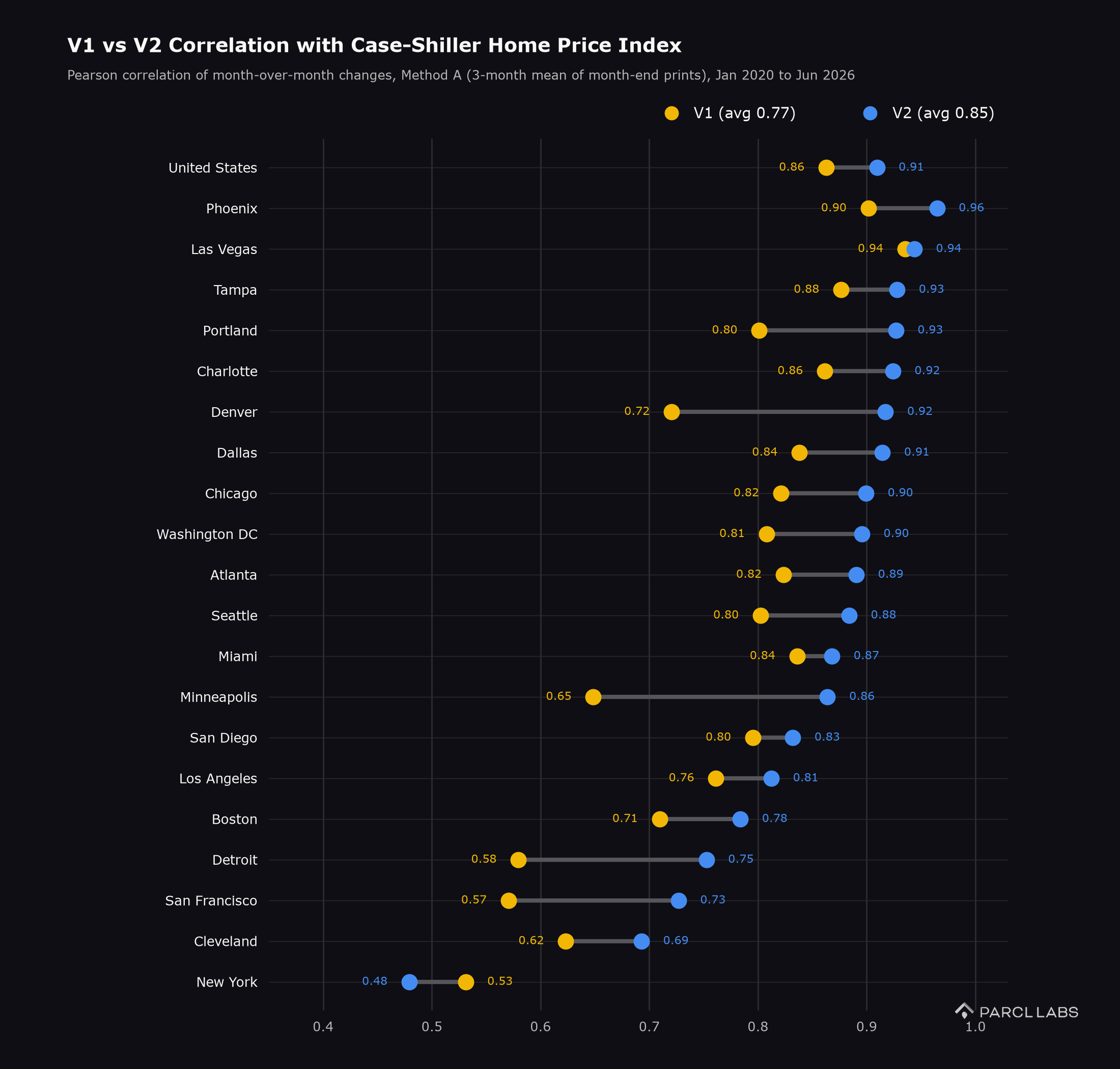
We also backtested the PLPF V2 against the Case-Shiller Home Price Index, a popular measure of home prices in the United States, and compared the result with our V1. Case-Shiller is a monthly index built as a three-month moving average, so we bring both versions of the daily feed to the same footing: we take the last print of each calendar month, average the latest three, and correlate the month-over-month change of that series with the month-over-month change of the Case-Shiller index for each of its twenty metropolitan areas and for the country, from January 2020 to June 2026. The PLPF V2 shows a higher degree of correlation with Case-Shiller than V1 in twenty of the twenty-one series, and the average correlation rises from 0.77 to 0.85, with the national series at 0.91. The largest gains come in markets such as Denver, Minneapolis, Detroit and San Francisco, where V1 had the least data to work with.

This agreement comes without the lag. Case-Shiller publishes more than two and a half months after the fact and is built only on repeat sales of single family homes. The PLPF V2 reads every home type, including condos, townhomes and new construction, and prints every day. A user gets a reading of the same market movement that Case-Shiller eventually confirms, months earlier and across tens of thousands of geographies rather than 20 markets.

Figure 3. Parcl Price Feed V1 and V2 Correlation with Case-Shiller Index

Conclusion

The PLPF V1 showed that a daily residential price feed was possible. The PLPF V2 takes that feed to every market and every segment: more than 40,000 daily price feeds across more than 20,000 U.S. geographies, from the ZIP code to the country, each broken into all homes, single-family homes and new construction. Where V1 read a few hundred markets as a single series, V2 reads the ZIP code, the city and the county, and separates the segments that move differently inside them. The markets that were hardest to measure, where transactions are sparse, records arrive late, or disclosed sale prices are incomplete, are now covered.

The PLPF V2 expands the markets it covers through dynamic look-back windows sized to each market's volume and a recency-weighted median that guards against sudden price movements. Instead of blending price levels, the feed chains daily returns, combining sales and listings as a weighted geometric mean of their movements. Working in log returns keeps gains and losses symmetric and lets each source contribute its movement without its level dominating, so the index stays tied to closed sales while moving with the freshest evidence. In thin markets we combine the market's own level with the movement of the geography that contains it, capturing real price movements in places with low volume.

For our users this means one accessible measure, a daily price per square foot, that reads the market and not the noise around it, and that can be compared across any two markets or segments because every feed is built the same way. Come an try it today on our API.